Case Study 8: Species Distribution Modeling with MaxEnt (Pseudo-Absence)
Predicting suitable habitats for a species using presence-only data and environmental variables by generating intelligent pseudo-absence points.
Introduction to Species Distribution Modeling
**Species Distribution Modeling (SDM)** is a technique used to predict the geographic distribution of species based on environmental conditions. **MaxEnt** (Maximum Entropy) is a popular machine learning algorithm for SDM, especially because it can work with **presence-only data** (locations where a species has been observed). However, to train a robust model, we also need locations where the species is likely absent. Since true absence data is often unavailable, we generate **pseudo-absence** points. This case study demonstrates an advanced method where we create pseudo-absences by identifying areas that are environmentally different from where the species is known to occur, leading to a more accurate and reliable habitat suitability map.
Analysis Workflow
1. Prepare Environmental Predictors
Load and process multiple environmental datasets (e.g., elevation, slope, NDVI, distance to forests/water) that are believed to influence the species' distribution.
2. Generate Pseudo-Absence Points
Use K-Means clustering to identify environmental zones. Sample points from zones where the species is not present to create a set of pseudo-absence points.
3. Combine Data and Train MaxEnt Model
Merge the known presence points (value 1) and the generated pseudo-absence points (value 0). Use this combined dataset to train the MaxEnt classifier.
4. Classify and Evaluate the Model
Apply the trained model to the environmental predictors to create a habitat suitability map. Evaluate the model's performance using the AUC (Area Under Curve) metric.
5. Analyze Variable Contributions
Generate a chart to determine the contribution of each environmental variable, identifying the most important factors driving the species' distribution.
Map Visualization
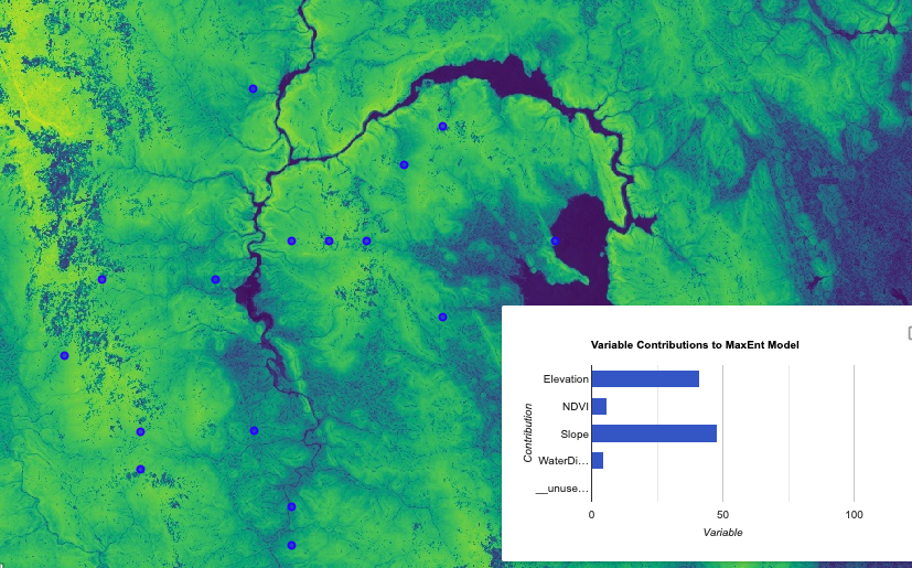
The final map shows the habitat suitability for the target species, ranging from low (purple/blue) to high (yellow/green). This continuous surface predicts the likelihood of finding the species based on environmental conditions.
GEE Code Snippet
This script prepares multiple environmental predictors, generates pseudo-absence points, trains a MaxEnt model, and evaluates its performance and variable contributions.
// NOTE: You must define a 'boundary' polygon and 'point' FeatureCollection before running.
var aoi = boundary;

// --- PREPARE PREDICTOR VARIABLES ---
var elev = ee.Image('NASA/NASADEM_HGT/001').select('elevation').clip(aoi);
var slope = ee.Terrain.slope(elev).rename('Slope');
var lulc = ee.Image("ESA/WorldCover/v100/2020").clip(aoi);
var imageCollection = ee.ImageCollection("LANDSAT/LC08/C02/T1")
                      .filterDate('2022-01-01', '2023-12-31')
                      .select(['B4', 'B5'],['RED','NIR']);
var ndvi = imageCollection.select('NIR').median().subtract(imageCollection.select('RED').median())
             .divide(imageCollection.select('NIR').median().add(imageCollection.select('RED').median()))
             .rename('NDVI').clip(aoi);
var distanceToWater = lulc.eq(80).fastDistanceTransform(30).sqrt().rename('WaterDistance');
var predictors = ee.Image.cat(ndvi, elev, slope, distanceToWater).unmask(0);

// --- GENERATE PSEUDO-ABSENCE and TRAIN MODEL ---
// This is a simplified representation of the complex function in the original script.
function PseudoAbsence(Point, Predictors, AOI){ /* ... (pseudo-absence logic) ... */ }
var PseudoPoint = PseudoAbsence(point, predictors, aoi);
var training = predictors.sampleRegions({collection: PseudoPoint, scale: 30});

// Define and train a Maxent classifier.
var classifier = ee.Classifier.amnhMaxent({randomTestPoints: 30, seed: 1}).train({
  features: training,
  classProperty: 'presence',
  inputProperties: predictors.bandNames()
});

// --- CLASSIFY AND VISUALIZE ---
var imageClassified = predictors.classify(classifier).clip(aoi);
Map.addLayer(imageClassified, {
  bands: ["probability"], max: 1.0, min: 0.0,
  palette: ["#440154FF", "#33638DFF", "#287D8EFF", "#55C667FF", "#DCE319FF"]},
  'Suitability Map');

// --- EVALUATE MODEL ---
var maxentExp = classifier.explain();
print('# Model Result', maxentExp);
var contribution = ee.Dictionary(maxentExp).get('Contributions');
var contributionChart = ui.Chart.feature.byProperty({features: ee.FeatureCollection(ee.Feature(null, contribution))})
  .setChartType('BarChart').setOptions({title: 'Variable Contributions'});
print(contributionChart);
print('# Training AUC:', ee.Dictionary(maxentExp).get('Training AUC'));
Analysis & Results
The analysis produces three critical outputs for understanding the species' habitat. First, the **Habitat Suitability Map** provides a continuous surface where colors like yellow and green indicate areas with high environmental suitability, while blue and purple indicate low suitability. This map is the primary prediction of where the species is most likely to be found.
Second, the **Variable Contributions Chart** is essential for ecological interpretation. It breaks down which environmental factors were most important for the model's prediction. For example, if 'Elevation' has the highest contribution, it tells us that elevation is a primary driver of this species' distribution. This insight is invaluable for conservation planning and understanding the species' niche.
Finally, the **Training and Testing AUC** values in the console provide a quantitative measure of model performance. The AUC (Area Under the Curve) score ranges from 0.5 (no better than random) to 1.0 (perfect prediction). A high testing AUC (typically > 0.8) indicates that the model is robust and has strong predictive power, giving us confidence in the suitability map.