Introduction to Above-Ground Biomass Estimation

**Above-Ground Biomass (AGB)** refers to the total mass of living organic matter in trees above the soil level, and it is a critical indicator of forest health, carbon storage, and ecosystem productivity. Direct measurement is difficult and costly, but we can estimate it using remote sensing. This case study uses data from the **Global Ecosystem Dynamics Investigation (GEDI)**, a Lidar instrument on the International Space Station that provides high-resolution measurements of forest vertical structure. By combining these accurate GEDI AGB point measurements with wall-to-wall satellite imagery from **Sentinel-2**, we can train a machine learning regression model (Random Forest) to predict and map AGB across an entire landscape.

Analysis Workflow

Map Visualization

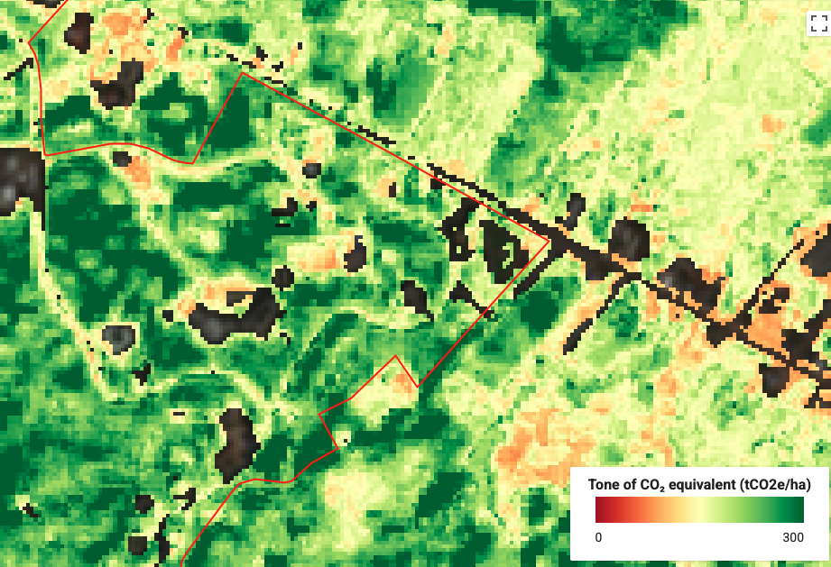
The final map shows the predicted Above-Ground Biomass Density (AGBD) in Megagrams per Hectare. The color ramp from light blue (low biomass) to dark green (high biomass) highlights the spatial distribution of carbon stocks within the forest.

GEE Code Snippet

This analysis is divided into three parts: data preparation, model training, and prediction/estimation.

Part 1: Data Preparation

// NOTE: You must define a 'geometry' polygon for your AOI.
// Load GEDI, Sentinel-2, and DEM collections.
var gedi = ee.ImageCollection('LARSE/GEDI/GEDI04_A_002_MONTHLY');
var s2 = ee.ImageCollection('COPERNICUS/S2_SR_HARMONIZED');
var glo30 = ee.ImageCollection('COPERNICUS/DEM/GLO30');
var startDate = ee.Date.fromYMD(2022, 1, 1);
var endDate = startDate.advance(1, 'year');

// Prepare Sentinel-2 composite with spectral indices.
var s2Composite = /* ... (cloud masking and index calculation logic) ... */;

// Prepare DEM and slope bands.
var elevation = glo30.filterBounds(geometry).mosaic().rename('dem');
var slope = ee.Terrain.slope(elevation);
var demBands = elevation.addBands(slope);

// Filter GEDI data for high quality measurements.
var gediMosaic = gedi.filterDate(startDate, endDate).filterBounds(geometry)
  .map(/* ... (quality, error, and slope masking) ... */)
  .mosaic().select('agbd');

// Export pre-processed data as assets.
Export.image.toAsset({image: s2Composite.clip(geometry), /* ... */});
Export.image.toAsset({image: demBands.clip(geometry), /* ... */});
Export.image.toAsset({image: gediMosaic.clip(geometry), /* ... */});

View Code (Part 1)

Part 2: Model Training

// Import assets from Part 1.
var s2Composite = ee.Image(exportPath + 's2_composite');
var demBands = ee.Image(exportPath + 'dem_bands');
var gediMosaic = ee.Image(exportPath + 'gedi_mosaic');

// Resample all data to a common 100m grid.
var stacked = s2Composite.addBands(demBands).addBands(gediMosaic);
var stackedResampled = stacked.reduceResolution({reducer: ee.Reducer.mean(), maxPixels: 1024})
  .reproject({crs: 'EPSG:3857', scale: 100});

// Use stratified sampling to get training points from GEDI pixels.
var training = stackedResampled.addBands(stackedResampled.select('agbd').mask().rename('class'))
  .stratifiedSample({numPoints: 1000, classBand: 'class', /* ... */});

// Train a Random Forest regression model.
var model = ee.Classifier.smileRandomForest(50)
  .setOutputMode('REGRESSION')
  .train({features: training, classProperty: 'agbd', /* ... */});

// Generate and print a chart of observed vs. predicted values.
var chart = ui.Chart.feature.byFeature({/* ... */});
print(chart);

// Classify the image to predict AGB.
var predictedImage = stackedResampled.classify({classifier: model, outputName: 'agbd'});
Export.image.toAsset({image: predictedImage, /* ... */});

View Code (Part 2)

Part 3: Estimation

// Import assets from previous parts.
var predictedImage = ee.Image(exportPath + 'predicted_agbd');

// Use a land cover map (ESA WorldCover) to mask non-vegetated areas.
var worldcover = ee.ImageCollection('ESA/WorldCover/v200').first();
var landCoverMask = worldcover.eq(10) // Forests
  .or(worldcover.eq(20)) // Shrubland
  .or(worldcover.eq(30)) // Grassland
  // ... (add other relevant classes)

var predictedImageMasked = predictedImage.updateMask(landCoverMask);
Map.addLayer(predictedImageMasked, gediVis, 'Predicted AGBD (Masked)');

// Calculate total AGB in Megagrams.
var pixelAreaHa = ee.Image.pixelArea().divide(10000);
var predictedAgb = predictedImageMasked.multiply(pixelAreaHa);
var stats = predictedAgb.reduceRegion({
  reducer: ee.Reducer.sum(),
  geometry: geometry,
  scale: 100,
  maxPixels: 1e10
});
var totalAgb = stats.getNumber('agbd');
print('Total AGB (Mg)', totalAgb);

// Convert to total Carbon.
var totalC = totalAgb.multiply(0.47);
print('Total Carbon (Mg)', totalC);

View Code (Part 3)

Analysis & Results

Reference