Case Study 2: Weather Interpolation for Data-Scarce Regions
Estimating spatial precipitation patterns from sparse weather station data using Inverse Distance Weighting (IDW) and Kriging interpolation methods.
Introduction to Weather Interpolation
Weather stations provide highly accurate climate data, but only for a single point. In many forested regions, especially in complex terrain, stations are sparse. **Interpolation** is a geostatistical method used to estimate values for an entire area based on a limited number of sample points. This is crucial for creating continuous climate surfaces, like a rainfall map, which are essential for hydrological modeling, species distribution modeling, and assessing drought risk in forests. This case study will compare two common interpolation techniques, **Inverse Distance Weighting (IDW)** and **Kriging**, to create a precipitation map for Northern Thailand.
Analysis Workflow
1. Define Area of Interest (AOI)
Isolate the provinces of Northern Thailand from an administrative boundary dataset to create a precise boundary for the analysis.
2. Load Weather Station Data
Create a `FeatureCollection` of point geometries representing weather stations, with annual precipitation as a property for each point.
3. Perform Interpolation
Apply both the Inverse Distance Weighting (`inverseDistance`) and Kriging (`kriging`) algorithms to the station data to generate two continuous raster surfaces.
4. Visualize and Compare
Clip both interpolation results to the Northern Thailand boundary and display them on the map using a shared color palette for direct comparison.
Map Visualization
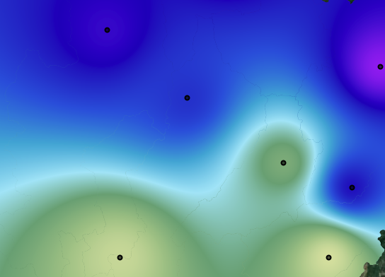
The map below shows the interpolated annual precipitation across Northern Thailand. The color gradient from white/yellow (drier) to dark blue/purple (wetter) reveals the estimated spatial patterns of rainfall.
GEE Code Snippet
This script defines a boundary, creates weather station points, and performs two types of spatial interpolation (IDW and Kriging) to estimate precipitation.
// -------------------- STEP 1: DEFINE NORTHERN THAILAND BOUNDARY --------------------
Map.setCenter(99.5, 18.5, 7);
var thailand_admin = ee.FeatureCollection("FAO/GAUL/2015/level1")
  .filter(ee.Filter.eq('ADM0_NAME', 'Thailand'));
var northernProvinces = [
  'Chiang Mai', 'Chiang Rai', 'Lampang', 'Lamphun', 'Mae Hong Son',
  'Nan', 'Phayao', 'Phrae', 'Uttaradit', 'Tak', 'Sukhothai',
  'Phitsanulok', 'Phetchabun', 'Kamphaeng Phet'
];
var northernThailand = thailand_admin.filter(ee.Filter.inList('ADM1_NAME', northernProvinces));
var maskRegion = northernThailand.geometry();

// -------------------- STEP 2: WEATHER STATION DATA --------------------
var stations = ee.FeatureCollection([
  ee.Feature(ee.Geometry.Point([99.50, 18.80]), {precip_mm: 1365}),
  ee.Feature(ee.Geometry.Point([100.25, 18.32]), {precip_mm: 1280}),
  ee.Feature(ee.Geometry.Point([98.98, 17.62]), {precip_mm: 1250}),
  ee.Feature(ee.Geometry.Point([99.82, 19.91]), {precip_mm: 1390}),
  ee.Feature(ee.Geometry.Point([100.60, 17.62]), {precip_mm: 1245}),
  ee.Feature(ee.Geometry.Point([101.00, 19.03]), {precip_mm: 1400}),
  ee.Feature(ee.Geometry.Point([100.78, 18.14]), {precip_mm: 1375}),
  ee.Feature(ee.Geometry.Point([98.88, 19.30]), {precip_mm: 1385})
]);
var meanStats = stations.reduceColumns({ reducer: 'mean', selectors: ['precip_mm'] });
var stdStats = stations.reduceColumns({ reducer: 'stdDev', selectors: ['precip_mm'] });

// -------------------- STEP 3: INTERPOLATION --------------------
var draftIDW = stations.inverseDistance({
  range: 1e6, propertyName: 'precip_mm', mean: meanStats.get('mean'), stdDev: stdStats.get('stdDev')
});
var draftKriging = stations.kriging({
  propertyName: 'precip_mm', shape: 'exponential', range: 1e6,
  sill: 1.0, nugget: 0.1, maxDistance: 1e6, reducer: 'mean'
});
var IDW = draftIDW.clip(maskRegion);
var Kriging = draftKriging.clip(maskRegion);

// -------------------- STEP 4: VISUALIZATION --------------------
var visParams = {
  min: 1200, max: 1400,
  palette: ['#ffffcc', '#c7e9b4', '#7fcdbb', '#41b6c4', '#2c7fb8', '#253494']
};

// -------------------- STEP 5: ADD LAYERS TO MAP --------------------
Map.addLayer(Kriging, visParams, 'Kriging Interpolation');
Map.addLayer(IDW, visParams, 'IDW Interpolation');
Map.addLayer(stations, {color: "black"}, "Weather Stations");
Map.addLayer(northernThailand.style({fillColor: '00000000', color: 'black'}), {}, "Northern Thailand Boundary");
Analysis & Results
The resulting maps display two different estimates of the spatial distribution of annual precipitation. Both methods show higher rainfall in the northernmost provinces like Chiang Rai and Mae Hong Son, and comparatively drier conditions in the central and southern parts of the region.
A visual comparison reveals key differences. The **IDW** map often produces a "bull's-eye" effect, with distinct circles of influence around each weather station. The **Kriging** map, a more advanced geostatistical method, typically produces a smoother and often more realistic surface because it considers the spatial autocorrelation of the data (how points closer together are more related than points farther apart).
For forestry, these interpolated surfaces are critical. They allow managers to move beyond station-specific data to understand landscape-level patterns. This can inform decisions about which tree species to plant based on water requirements, identify areas at higher risk of drought-induced stress, and improve inputs for models that predict forest growth and water yield from forested catchments.